
In this article, we start with the basics of probability. Loosely speaking, probability is a systematic way of dealing with uncertainty. Real world is uncertain, for example, there can always be some sort of noise when signal is transmitted from once place to another. Another example can be, the life of our cellphone is uncertain where it may range from one (or even less) year to many years. Probabilistic frameworks deal with modeling such kind of uncertainty. It has applications in the many disciplines of engineering and science. However, the underlying principles of probability remain same for all the discipline. So let’s start with basics of this fascinating area.
Let’s discuss each of the components separately.
Before that let’s introduce some terminology.
: It can be anything such as tossing a coin, playing a match, rolling a dice, etc.
An experiment one or more outcomes. An outcome is the result of that experiment For example, cricket match between India and Pakistan is an experiment and its outcomes for a team can be (win, loose, tie, forfeit). Other examples of an experiment are rolling a dice or tossing a coin. In case of tossing a coin what are the possible results? It will be either head or tail (if you are unlucky it may get stuck in between J ), right? In case of rolling a dice (6 faced), the possible results are getting 1 or 2 or 3, or 4, or 5 or 6). So, for modeling any probabilistic model, first of all we should define its all possible outcomes. This list is called sample space. All these experiments have uncertainty, that’s why we model them using probability.
It is important to remember that, no matter what happens only one element of this list happens. i.e., either a team wins or loses, a team cannot win and loses a same match at the same time. Either head or tail occurs, both cannot occur at the same time. In simple words, if one outcome happens other cannot happen at that time. Moreover, we are certain that once of elements of the sample will always occur. i.e., there will always be the result of cricket match where win, loose, tie or forfeit. There will always be a head or tail if we toss a coin (no third option).
What about our initial beliefs? I am going to toss a coin and ask you, will it be a head or tail? Assuming that you don’t have an access to future results you cannot predict. It can be either head or tail. If I ask you chances of head are more than tail? Again, we cannot tell in advance. So our initial belief about the toss of coin is: Both head and tail have equal chances to occur. Now what is your initial belief about the rolling of a dice? Again, any number between 1 and 6 can be the outcome of the event. So these are our initial beliefs.
Let’s elaborate parts b) and c). If a team either wins or loses (for simplicity, let’s keep only these two outcomes), then if 60% (60/100 which makes 0.6) chances are their win then 40% (0.4) chances will be their loosing, which makes a total of 100% (0.6+0.4=1). It cannot happen that a team has 60% chance of win and 60% chance of losing.
One more example, in case of roll of a dice, total probability is: P(S) = P(1) + P(2) + P(3) + P(4) + P(5)+ P(6).
Now I ask you, what is the probability of getting 1? The answer is P(1) = 1/6.
Now I ask you, what is the probability of getting 3? The answer is P(3) = 1/6 .
Now I ask you, what is the total probability of getting 1 or getting 3?
The answer is (using additivity rule): P(1 U 3) = P(1) + P(3)= 1/6 + 1/6 = 2/6=1/3
It is important to note that additivity axiom does not only apply to two sets A or B. If we have more than two set, same axiom can be extended. i.e.,
P (A U B U C U D) = P(A) + P(B) + P(C) + P(D)
I above examples we had a finite or defined set of outcomes (head or tail), (win, loose, tie, forfeit). These finite outcomes are called the discrete sample space. Now if I ask, what is the list of pair two numbers (x,y), where both x and y can be between 0 and 1. A few examples of such list are:
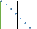
(0,0), (0.001, 1), (0.000001,1), (1,0), (1, 0.000000001), and so on. So in this example, we have infinite number of such pairs between 0 and 1. We call such an infinite sample space as continuous or infinite sample space. Now, I ask, what is the probability or chance of getting an exact pair (0, 0001)? It is very small. Hence in case of continuous sample space, instead of assigning probabilities to individual outcomes, we assign probability of a subset. Let’s illustrate it with another example: The probability of hitting any individual small blue dot in the square given below is very small. So instead of assigning an individual outcome, we divide the square into two parts (or subsets). These subsets are 1) the left side of the black line and 2) the right side of black line. Now, the probability of falling on the left side is much larger than hitting the probability of hitting an individual dot. The point I want to make is, in case of continuous sample space, probabilities are assigned to subsets, not individual outcomes (because they are very small).
In this article, I discussed some of the basics of probability. We define an experiment, its outcomes. Then we introduced sample space, as well as axioms of the probability. We also categorized the sample space into discrete and continuous classes. I hope you enjoyed this article.
Powered by Froala Editor