

One of the most interesting and popular subfields of artificial intelligence is computer vision. A computer can analyze and comprehend visual input from its surroundings by using a set of instructions called a computer vision algorithm. These algorithms may be applied to a variety of tasks, including object detection, image classification, facial recognition, and video tracking. Images and videos are analyzed and processed by using these algorithms. Computer vision methods are revolutionizing businesses worldwide, whether it is finance, agriculture, healthcare, automotive, security or facial recognition. The goal of computer vision is to make the machines able to recognize and interact with things in images and videos in the same manner that humans do. In certain tasks, such as object detection and labelling, computer vision algorithms have outperformed humans in terms of speed and accuracy. We'll study some of the most well-known computer vision algorithms in this article, along with some of their intriguing uses.
In his 2004 publication, Distinctive Image Features from Scale-Invariant Keypoints, D. Lowe of the University of British Columbia developed a novel technique called Scale Invariant Feature Transform (SIFT) that extracts keypoints and computes its descriptors in an image. The SIFT method is used to recognize and match local features in images, such blobs or corners, referred to be the "keypoints" of the image. It identifies important locations and provides them with quantitative data, also referred to as descriptors, which are utilized in object detection and recognition. The descriptors that are acquired via the use of SIFT are resistant to perspective, rotation, and lighting changes, allowing the picture to appear different even while the objects are the same. After then, these descriptors may be applied to tasks such as object identification, image retrieval, and image matching. The rotation and size of the image have no effect on the SIFT technique.
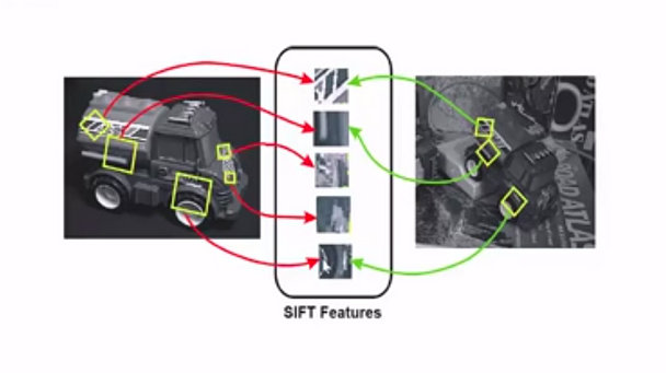
It makes sense to humans that although the thing in the image may alter in size or angle, it stays the same. However, machines struggle greatly with the same concept. If we alter some aspects of an image, such as the angle or size, it becomes more difficult for machines to identify the item. The robots can be trained to recognize images nearly as well as humans can because of their extreme flexibility.
There are mainly four steps in SIFT computer vision algorithm:
1. Scale-space Extrema Detection
We must find the most distinguishing characteristics in a given input image with noise ignored. We also need to make sure that the characteristics are independent of scale. Using a difference-of-Gaussian, or DoG, function, the algorithm examines the whole image and scales in order to find possible interest points. Both scale and orientation have no effect on these locations.
Gaussian Blur
We apply the Gaussian Blurring method in an image to reduce the noise. The Gaussian Blur uses a given sigma value to compute a value for each pixel in an image depending on its nearby pixels.
Gaussian Blur assist with image processing, effectively removes noise from the photos when the key elements from the image are highlighted. Then, we must confirm that these features rely on scale. This implies that by establishing a "scale space," we will be looking for these properties on several sizes and multiple scales.
A set of images with varying scales that are produced from a single image is called a scale space.
The blurry pictures are therefore created for various scales. We will take the original image and cut the scale in half to generate a new collection of images at different scales. For every new image, a blur version will be created.
Difference of Gaussian (DoG)
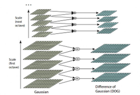
The images with various scales (often denoted by σ) will be produced and applied Gaussian blur to each one in order to minimise image noise. We will then make an effort to improve the features by applying a method known as the Difference of Gaussians, or DoG.
The Difference of Gaussian method is a feature improvement technique that require subtracting a blurry original image version from a less blurry original image version.
DoG subtracts each image from the preceding image in the same scale to produce a new collection of images for each octave. Below is given a diagram that illustrates the implementation of DoG:
2. Keypoint Localization
Once the images have been prepared, finding the keypoints in the image that may be utilized for feature matching comes next. The goal is to locate the local maxima and minima for the images. There are two phases in this section:
Local Maxima and Local Minima
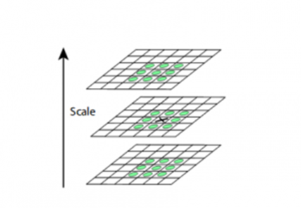
We go over each pixel in the image and compare it with its neighbouring pixels to find the local maxima and minima. When the term "neighbouring" is used, it’s not mean just the pixels that surround the pixel in image but also the nine pixels that make up the preceding and next image in the octave. This implies that in order to determine if a given pixel value is the local maximum or minimum known as extrema, it is compared to 26 other pixel values.
For instance, the illustration below shows three images from the first octave. If the pixel with the symbol x is the highest or lowest among its neighbours, it is compared to the neighbouring pixels (shown in green) and designated as a keypoint or interest point:
Keypoint Selection
The keypoints that are too close to the edge or have poor contrast will be removed.
For every keypoint, a second-order Taylor expansion is calculated in order to address the low contrast keypoints. The keypoint is rejected if the final value (in magnitude) is less than 0.03 (as per the paper).
3. Orientation Assignment
We now have a set of reliable keypoints for the images. In order to make each of these keypoints rotationally invariant, we will now assign them an orientation. We may split this process again into two more smaller steps:
4. Keypoint Descriptor
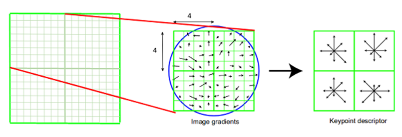
This completes the computer vision process for SIFT (scale invariant feature transform). Up to this point, we have rotationally and scale-invariant stable keypoints. In this part, we will generate a distinct fingerprint for this keypoint, known as a "descriptor," using the neighbouring pixels, their orientations, and their magnitude.
Furthermore, the descriptors will be partially invariant to the lighting or brightness of the pictures since we use the surrounding pixels.
The keypoint descriptor has now been created. The keypoint's 16x16 neighbourhood is seized. It is divided into sixteen 4x4 size subblocks. An 8 bin orientation histogram is created for every sub-block. Thus, total 128 bin values are accessible. To make a keypoint descriptor, it is expressed as a vector. Furthermore, other steps are implemented to attain resilience against illumination variations, rotation, and other factors.
5. Feature Matching
Now, we will match features using the SIFT computer vision features. The keypoints in two images are matched by locating their closest neighbours. However, the second closest match could occasionally be very close to the first. It might occur as a result of noise or another factor. The distance ratio of closest-to-second-closest distance is then calculated. If it exceeds 0.8, they are dismissed. According to the paper, it eliminates over 90% of erroneous matches and discards just only 5% of true results.
SURF is a novel method that was first proposed in a work titled "SURF: Speeded Up Robust Features" published in 2006 by three people: Bay, H., Tuytelaars, T., and Van Gool, L. The SURF is an algorithm for detecting and describing features in images. It is an efficient fast technique that is frequently utilized in computer vision applications like image registration, object detection, classification, and reconstruction tasks. It is believed that the Scale-Invariant Feature Transform (SIFT) method has been "speeded up" by SURF. For real-time applications, it is more beneficial than SIFT because of its computational efficiency.
A computer vision algorithm called SURF has 2 steps:
Feature Extraction: It involves choosing an interest point in the image by approximating it using a Hessian matrix.
Feature Description: There are two phases involved in creating the SURF descriptor. First, using the circular space information surrounding the keypoint (interest point), we determine an orientation. Then, we build a square area that is in line with the orientation so that the descriptors may be extracted.
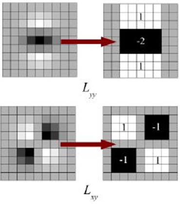
Lowe estimated the Laplacian of Gaussian with Difference of Gaussian for the purpose of determining scale-space in SIFT. SURF uses a Box Filter to simulate LoG.An example of such an approximation may be seen in the image below. Squares have been used as an approximation in place of a Gaussian average of the images. This produces better results since using the integral image speeds up convolution with squares. This method of approximation has the major benefit of making convolution with a box filter simple to compute using integral images.Moreover, it may be completed in parallel at various scales. Additionally, the SURF depends on the Hessian matrix determinant for both location and scale.
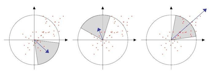
SURF employs wavelet responses in both the horizontal and vertical directions for orientation assignment for a neighborhood with a size of 6. It also has appropriate gaussian weights added to it. Integral images make it relatively simple to determine the wavelet response at any scale. This orientation does not need to be found because rotation invariance is not required for many applications, which speeds up the procedure. One such feature offered by SURF is known as Upright-SURF, or U-SURF. Wavelet responses are used by SURF in both the horizontal and vertical directions (again, using integral pictures makes things simpler), this gives feature description. The keypoint is surrounded by a neighbourhood of size 20sX20s, where s is the size. There are four 4x4 subregions in it. Wavelet responses are obtained in both horizontal and vertical directions for each subregion, and a vector is created.This produces SURF feature descriptor with 64 dimensions when expressed as a vector. Reduced dimension results in faster matching and computing speed, but improved feature uniqueness.
During the detection phase, the Laplacian sign is calculated and utilised for underlying interest positions. In images, the Laplacian sign helps to identify bright blobs on dark backgrounds. Images are only compared for matching if their features have the same kind of contrast according to the orientation sign. This makes faster matching possible.
Advantages of SURF Algorithm:
When it comes to real-time computer vision applications, SURF outperforms SIFT. It is also less dimensional and requires less computing time.
Disadvantages of SURF Algorithm:
Rotation is not stable for SURF. If there are issues with the images' lighting, it does not operate as expected.
The Viola-Jones object identification method was created by two computer vision researchers Paul Viola and Michael Jones in 2001 to address the face detection issue. Real-time image detection is made possible by it. Although it takes a bit longer time for this method to train on a particular dataset but it is capable of real-time face detection with exceptional speed and accuracy. The Viola-Jones algorithm recognises faces in images by using Haar-like characteristics.
The Viola-Jones algorithm consists of four key steps: given a picture (colour or grayscale), the algorithm looks at numerous smaller subregions within the image and searches each subregion for particular features in an attempt to identify a face. An image may have several faces of varying sizes, therefore the algorithm must verify a wide range of scales and locations.
1. Haar-like Features:
It has the name after Alfred Harr, Hungarian mathematician who created the idea of Haar wavelets.
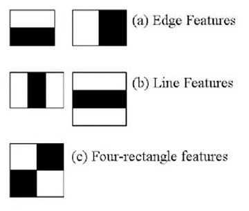
The features display a box with two sides, a bright and a dark one, which is how the machine recognises a feature.
Viola and Jones identified three categories of Haar Features, which are:
Edge Features
Line Features
Four Rectangle Features/ Four-sided features
2. Integral Images:
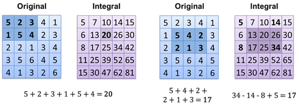
Each point in an integral image is equal to the total of all pixels to the left and above, including the target pixel.
3. Adaptive Boosting (AdaBoost) Training:
We give the information to the classifier during training so that it may learn from the data and make predictions. In the end, the algorithm sets a minimal threshold for determining whether anything classifies as a feature or not.
The image's size is reduced to 24 x 24 pixels during the training phase, and features are found within the image. For the algorithm to be trained, a large amount of image data is required. Viola and Jones provided 4960 manually labelled photos to feed their algorithm. In order to help the classifier understand and categorise, we should also provide it with non-facial photos. Viola and Jones provided 9,544 non-facial images for their algorithm.
By using the images we provide from the training dataset, the algorithm improves its precision and accuracy by identifying true negatives and false positives in the dataset. Once we have examined every possible location and feature combination, we have an accurate model.
4. Cascade of Classifiers:
Cascading provides an additional technique to improve the algorithm's speed and accuracy. Every level in cascading has a powerful classifier. Every feature is grouped into many phases. Every stage has a number of features. The task of each step is to determine whether a certain sub-window in an image is a face or not. If at any point a sub-window is unable to identify a face, it is instantly dismissed as not being a face.
In computer vision, object detection is a method used to localize and identify onjects inside an image or video.
The technique of finding one or more items correctly using bounding boxes which correlate with rectangular shapes that surround the objects is known as image localization.
Image recognition or classification attempts to identify which category or class an image or object inside an image belongs to.
What is YOLO?
You Only Look Once (YOLO), an innovative real-time object identification system was announced in 2015 by Joseph Redmon, Santosh Divvala, Ross Girshick, and Ali Farhadi in their well-known academic work "You Only Look Once: Unified, Real-Time Object Detection".
By establishing spatially separated bounding boxes and allocating probabilities for all of the detected images using a single convolutional neural network (CNN), the authors modify the object identification problem as a regression problem rather than a classification assignment.
YOLO, or You Only Look Once, is a very quick multi-object identification method that makes use of convolutional neural networks (CNNs) to recognize and identify items. Furthermore, when compared to comparable real-time systems, YOLO achieves more than double the mean Average Precision (mAP), making it an excellent choice for real-time processing.
With very few background mistakes, YOLO's accuracy much exceeds than that of other advanced models.
The neural network has this network architecture.
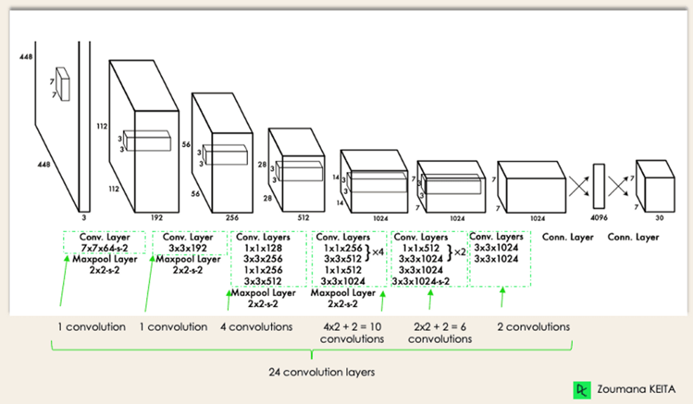
The architecture functions as:
Before the input image is processed by the convolutional network, it is resized to 448 × 448.
To produce a cuboidal output, a 3x3 convolution is used after a 1x1 convolution to lower the number of channels.
The base activation function is ReLU, with the exception of the final layer, which employs a linear activation function.
Some additional approaches, such dropout and batch normalisation, regularise the model and keep it from overfitting, respectively.
How Does YOLO Object Detection Work?
Whole process of how YOLO performs object detection; how to get image (B) from image (A)”
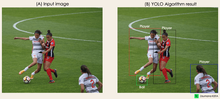
The algorithm operates using the four strategies listed below:
1. Residual blocks
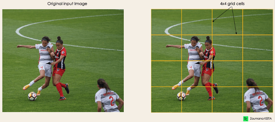
In the first phase, the original picture (A) is divided into NxN grid cells of equal shape (the figure on the right shows N as 4 in our example). The task assigned to each grid cell is to locate the object it covers, predict its class, and provide the probability and confidence value for that class.
2. Bounding box regression
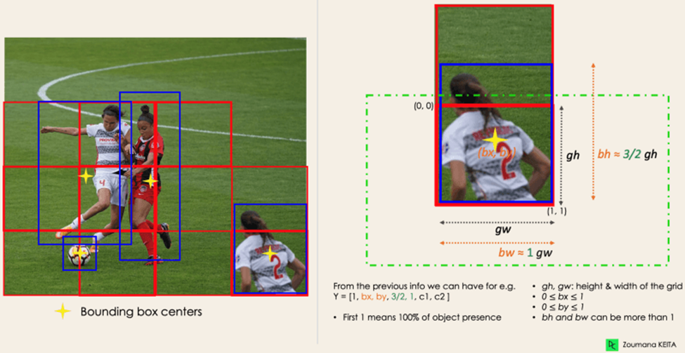
The next step is finding the bounding boxes, which match the rectangles indicating each object in the image. Bounding boxes can be added to an image in an equal number as the number of items it contains.
YOLO uses a single regression module to determine the properties of these bounding boxes, where Y is the final vector representation for each bounding box.
Y = [pc, bx, by, bh, bw, c1, c2]

Let's take a closer look at the player on the bottom right:
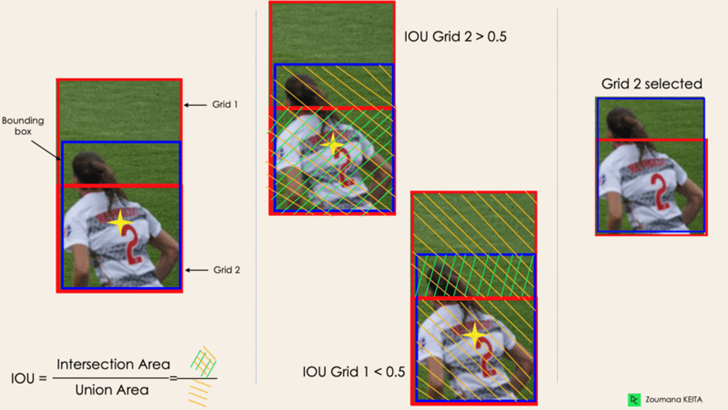
3. Intersection Over Unions or IOU
Many times, even though not all of them are significant, a single item in an image can have many grid box possibilities for prediction. The IOU, which has a value between 0 and 1, aims to eliminate these grid boxes and retain just the ones that are meaningful.
An example of using the grid selection procedure on the bottom left object is shown below. It is evident that only "Grid 2" was ultimately chosen out of the two grid possibilities which the object initially possessed.
4. Non-Maximum Suppression (NMS)
An object may contain several boxes with IOU beyond the threshold, and leaving all those boxes might include noise, therefore setting a threshold for the IOU is not necessarily sufficient. This is the point when we can apply NMS to retain just the boxes that have the greatest detection probability score.
Conclusion:
This article has covered the computer vision algorithms compared among different object detection algorithms, and their evolution.
Although computer vision is difficult and takes a lot of work to begin exploring, deep learning techniques allow us to solve difficult computer vision issues like image classification, detecting objects, and face recognition using advanced technology.
It is concluded that YOLO's quick progress means that it will undoubtedly hold the top spot in the object detection sector for a very long time.
References:
https://docs.opencv.org/4.x/da/df5/tutorial_py_sift_intro.html
https://docs.opencv.org/4.x/df/dd2/tutorial_py_surf_intro.html
https://docs.opencv.org/4.x/d2/d99/tutorial_js_face_detection.html
https://towardsdatascience.com/viola-jones-algorithm-and-haar-cascade-classifier-ee3bfb19f7d8
https://towardsdatascience.com/the-viola-jones-algorithm-7357c07d8356
https://opencv-tutorial.readthedocs.io/en/latest/yolo/yolo.html
https://www.datacamp.com/blog/yolo-object-detection-explained