


In recent times, we have seen a great possibility in applying artificial intelligence (AI) in weather forecasting, especially when it comes to better flood prediction and handling. This paper studies how AI can be used to lessen the effects of monsoon floods in Pakistan - an area often hit by severe weather. It uses data on rainfall from 2019 to 2023. It uses multiple techniques such as time series analysis, ARIMA models, and high-end machine learning methods for better flood prediction.
This work's primary goal is to create a model that can predict heavy rains more accurately. This will help in giving early warnings about floods and getting prepared in advance. The methods include processing and analyzing data, forecasting using time series, and using SARIMA models with auto-ARIMA for better predictions. Besides, this paper also discusses the importance of refining the model's accuracy by optimizing hyperparameters using the Firefly Algorithm.
The findings of this study show that models powered by AI can significantly improve monsoon rain forecasts. They provide an important aid for groups that deal with disasters. By giving correct predictions at the right times, these models help lower the bad effects of floods and increase resilience against monsoon rains within communities residing in Pakistan.
The weather data for this study was meticulously gathered from multiple reliable sources, including local meteorological departments and global weather databases. This dataset encompasses detailed records spanning several years, providing a comprehensive view of the weather patterns. By consolidating data from various sources, a robust dataset was assembled, capturing essential weather variables necessary for in-depth analysis.
Feature | Description |
name | The location where the weather data was recorded. In this dataset, the location is 'lahore' |
date | The date of the observation, formatted as DD/MM/YYYY. Provides the temporal context for each recorded measurement. |
Time | The time of the observation, formatted as HH . Specifies the exact hour at which the weather data was recorded. |
Temp | The temperature in degrees Celsius at the time of observation. Provides information on thermal conditions. |
Dew | The dew point in degrees Celsius, indicating the temperature at which air becomes saturated with moisture. |
Humidity | The relative humidity percentage, representing the amount of moisture in the air relative to the maximum amount the air can hold at that temperature. |
precip | The amount of precipitation in millimeters recorded during the observation period. Crucial for analyzing rainfall. |
Preciptype | The type of precipitation observed (e.g., rain, snow, etc.). Categorizes the form of precipitation recorded. |
Windgust | The maximum wind gust speed in kilometers per hour recorded during the observation period. Indicates the strongest wind bursts. |
Windspeed | The average wind speed in kilometers per hour during the observation period. Provides information on general wind conditions. |
Winddir | The direction of the wind in degrees. Shows the compass direction from which the wind is blowing. |
sealevelpressure | The atmospheric pressure at sea level, measured in millibars. Provides insight into overall pressure conditions. |
Cloudcover | The percentage of cloud cover in the sky. Indicates the extent of cloudiness and its impact on weather conditions. |
Conditions | A textual description of the general weather conditions, such as "Clear", "Partially cloudy", etc. Summarizes the weather situation. |
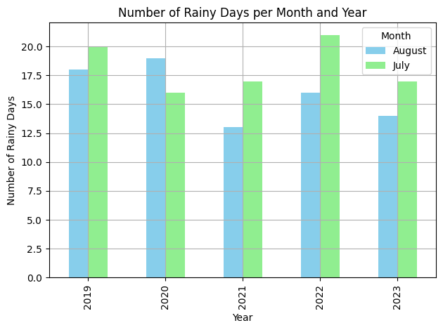
Number of Rainy Days per year and month
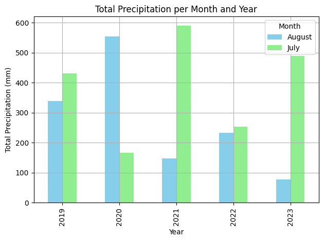 Total Precipitation per Month and Year.
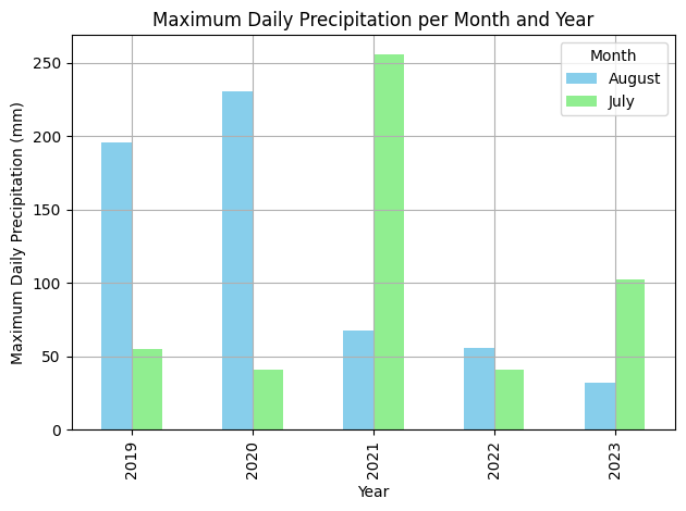 Maximum Precipitation per Month and Year
In our study, the ACF and PACF charts played a key role in setting the right parameters the ARIMA model. The ACF helps to gauge the correlation of rain amount values at differing lag times, which was fundamental in pinpointing the Moving Average (MA) element. Remarkable surges in the ACF chart were indicators of how many previous observations affected upcoming values. For example, surges up to lag 2 indicated an MA part of order 2.
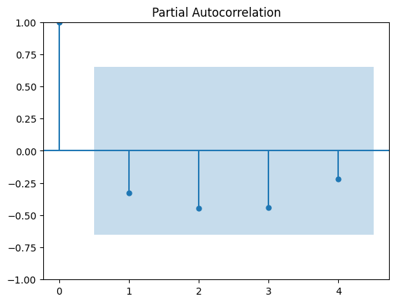
The PACF displays connections between rainfall amounts and their lags but excludes any influence from intermediate lags. This guides towards out an Auto-Regressive (AR) element. Significant height increases at certain lags on a PACF chart showed how many preceding observations should be incorporated into the model. For instance, a notable surge at lag 1 without any additional significant surges pointed towards an AR component of order 1.
Interpreting findings from both ACF and PACF charts helped fine-tune the ARIMA model leading to more precise rain forecasts.
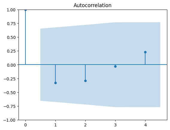 Autocorrelation Function (ACF)
 Partial Autocorrelation Function (PACF)
ARIMA (AutoRegressive Integrated Moving Average): In the context of flood prediction, ARIMA is used to model and forecast precipitation patterns based on historical rainfall data. The AR component leverages past precipitation values to predict future amounts, the I component ensures the time series is stationary by differencing the data, and the MA component corrects for any residual errors in the predictions. This model helps in understanding how past precipitation influences future rainfall and in predicting flood events based on historical trends.
SARIMA (Seasonal AutoRegressive Integrated Moving Average): SARIMA is particularly useful for capturing seasonal variations in rainfall data, which is crucial for accurate flood prediction. By adding seasonal AR and MA components, SARIMA can account for periodic
fluctuations in rainfall that occur at specific intervals (e.g., monsoon seasons). Seasonal differencing helps in making the time series stationary by removing these seasonal effects, which improves the model's ability to forecast flood events accurately during different seasons of the year.
Auto-ARIMA: Auto-ARIMA simplifies the process of model selection by automatically identifying the best ARIMA or SARIMA configuration for your data. It evaluates various combinations of parameters to find the most effective model for predicting precipitation. This automated approach enhances efficiency and reduces the risk of manual errors, allowing for more accurate forecasting of flood events based on historical data. By optimizing the model fitting, Auto-ARIMA ensures that the chosen model best captures the underlying patterns in the precipitation data.
1. Initialization:
Model Selection: We selected the ARIMA (AutoRegressive Integrated Moving Average) model to forecast future precipitation values based on historical data.
Parameter Choice: The parameters for ARIMA, denoted as (p,d,q), were chosen based on the ACF (AutoCorrelation Function) and PACF (Partial AutoCorrelation Function) plots. For this instance, we used (1,1,1), where:
p (AutoRegressive order) is 1.
d (Differencing order) is 1.
q (Moving Average order) is 1.
2. Training Execution:
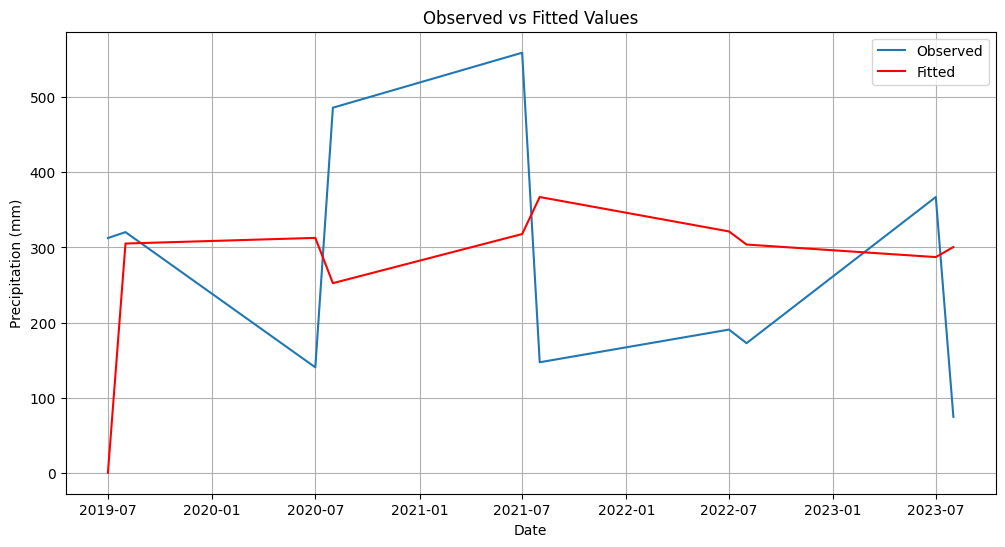
Model Fitting: The ARIMA model was trained on the monthly_data['precip'] series. This involved estimating the model parameters using the historical precipitation data to capture trends and seasonality.
Results Summary: After fitting the model, the model_fit.summary() function was used to obtain a detailed summary of the model’s performance, including coefficients, statistical significance, and model diagnostics.
 ARIMA Model Training
1. Initialization:
Model Selection: The SARIMA (Seasonal AutoRegressive Integrated Moving Average) model was chosen to account for both seasonal and non-seasonal components in the time series data.
Parameter Choice: For this instance, the SARIMA model was configured with:
Non-seasonal parameters: (p,d,q)=(1,1,1)
p: AutoRegressive order
d: Differencing order
q: Moving Average order
Seasonal parameters: (P,D,Q,s)=(1,1,1,12)
P: Seasonal AutoRegressive order
D: Seasonal Differencing order
Q: Seasonal Moving Average order
s: Seasonal period (12 for monthly data with annual seasonality)
2. Training Execution:
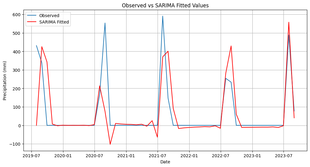
Model Fitting: The SARIMA model was trained on the monthly_data series. This involved fitting the model to account for both non-seasonal and seasonal components in the precipitation data.
Results Summary: The sarima_fit.summary() function was used to obtain a detailed summary of the model's performance, including parameter estimates, statistical significance, and model diagnostics.
3. Post-Training Evaluation:
Model Assessment: Review the model summary to evaluate the fit of the model. Key metrics such as AIC (Akaike Information Criterion) and BIC (Bayesian Information Criterion) are examined to assess the model's performance.
Residual Analysis: Analyze the residuals to ensure they exhibit white noise characteristics, indicating that the model has adequately captured the data's patterns.
 SARIMA Model Training
1. Initialization:
Model Selection: Auto-ARIMA was chosen to automate the selection of the best ARIMA or SARIMA model for the time series data.
Parameters Configuration:
Seasonal Component: Enabled to capture seasonal patterns in the data.
Seasonal Period (m): Set to 12, corresponding to monthly data with an annual seasonal cycle.
Trace: Enabled to provide detailed output during the model selection process.
Error Action: Set to 'ignore' to prevent the model from stopping due to errors.
Suppress Warnings: Enabled to reduce verbosity of warnings during model fitting.
2. Training Execution:
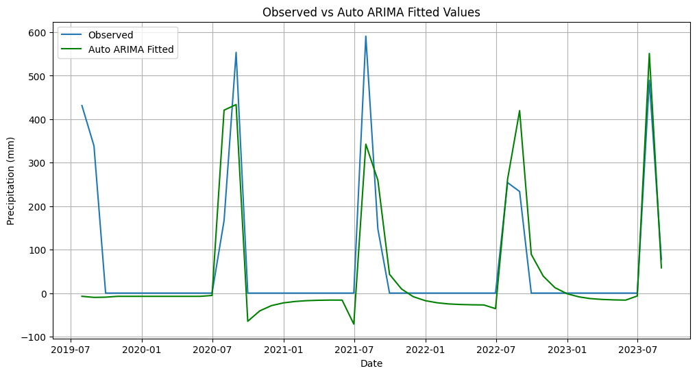
Model Fitting: The auto_arima function was used to automatically select the best combination of ARIMA or SARIMA parameters by evaluating various models based on performance metrics. The model was then fitted to the monthly_data series.
Results Summary: The auto_arima_model.fit() function provides a model fitted with the best parameters identified during the search process. This function also offers insights into the model selection process and chosen parameters.
3. Post-Training Evaluation:
Model Assessment: Review the output from auto_arima to understand the optimal parameters chosen and the performance of the selected model.
Diagnostics: Analyze the residuals and other diagnostics to confirm that the model effectively captures the underlying patterns in the data without significant errors.
 Auto ARIMA Model Training
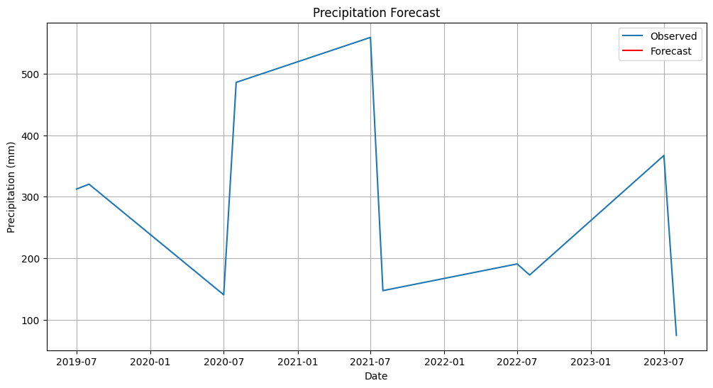 ARIMA Model Forecast Graph
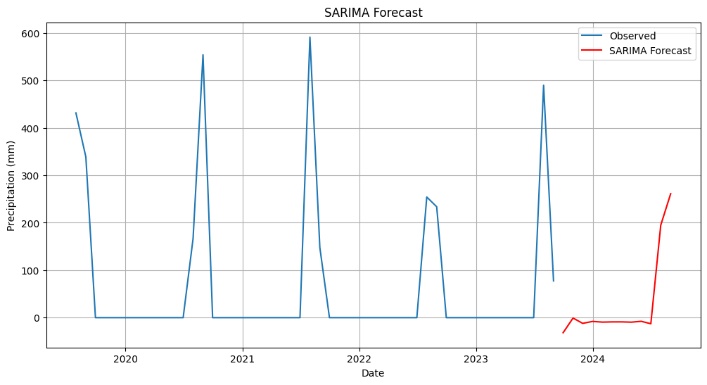 SARIMA Model Forecast Graph
Performance Matrix | Score |
Mean Absolute Error (MAE) | 146.392 |
Mean Squared Error (MSE) | 23761.09 |
Root Mean Squared Error (RMSE) | 154.14 |
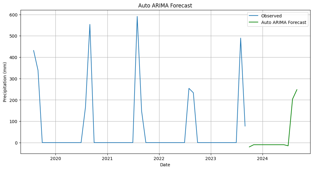 Auto ARIMA Model Forecast Graph
Performance Matrix | Score |
Mean Absolute Error (MAE) | 52.85 |
Mean Squared Error (MSE) | 10759.23 |
Root Mean Squared Error (RMSE) | 103.73 |
This study highlights the powerful role of artificial intelligence (AI) in improving flood prediction and management for monsoon floods in Pakistan. By leveraging advanced time series analysis and machine learning models like ARIMA, SARIMA, and Auto-ARIMA, we have developed models that significantly enhance the accuracy of rainfall forecasts.
Our results show that SARIMA and Auto-ARIMA models deliver more reliable predictions by capturing seasonal patterns and optimizing parameters, respectively. These AI-driven approaches outperform traditional methods, leading to better flood preparedness and mitigation. Accurate forecasts enable disaster management agencies to make timely, informed decisions, ultimately reducing the impact of monsoon floods on communities.
Model Enhancement: Continue to refine and enhance the AI models by integrating additional features, such as real-time weather data and geographical information, to improve prediction accuracy and adaptability.
Extended Dataset: Expand the dataset to include more years and diverse weather conditions. This will help in developing more robust models that can handle various scenarios and improve long-term forecasting.
Integration with Early Warning Systems: Implement AI models within existing early warning systems to provide real-time flood alerts and actionable insights. This integration can enhance the timeliness and effectiveness of flood management efforts.
Cross-Validation with Other Models: Explore and compare other advanced machine learning models, such as deep learning techniques, to assess their potential for better performance and accuracy in flood prediction.
User-Friendly Tools: Develop user-friendly tools and dashboards for stakeholders and disaster management agencies to easily access and interpret the predictions and insights generated by the AI models.
Collaborative Research: Foster collaboration between meteorologists, data scientists, and local authorities to ensure that AI models are continuously updated with the latest data and feedback, improving their relevance and effectiveness.
Powered by Froala Editor